|
|
|
3D Mandelbrot Generator |
|
|
|
3D Mandelbrot Generator. I've attempted many
times to create 3D Mandelbrot Sets with less
than satisfying results. In the standard
Mandelbrot Set, the iteration count
is used to pick a color from a palette. One way
to create a 3D Mandelbrot would be to use the
iteration count as an elevation or z-axis value.
This works reasonably well and with a little bit
of work, you get images like the one to the
right. On the other
hand, there is something unsatisfying about
these images. While they are fractal in two
dimensions, they are non-fractal and rather
plain in the third dimension. |
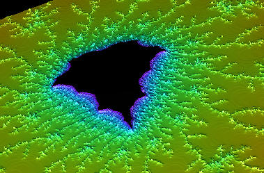
2D Mandelbrot Set
using color as the Z-dimension |
|
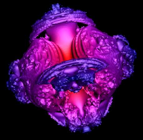
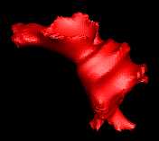
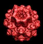
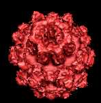
Real 3D Mandelbrot. That all changed when I
came across
Daniel White's web page. Daniel's web
page describes his own search for a true 3D
Mandelbrot and his discoveries. The ultimate
result is something that is now called the "Mandelbulb."
Daniel uses ray tracing to render
his 3D Mandelbrots, but I thought it would be
interesting to try OpenGL and 3D modeling. A 3D
model would have the advantage that you could
manipulate it in real time. The image to the
right shows an example of what I was able to
create. |
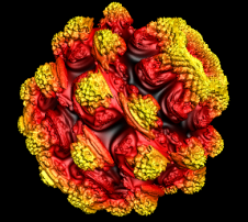
True 3D Mandelbrot set
The Mandel Bulb |
|
Image Gallery |
|
Mandel Bulb Images |
|
 |
|
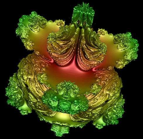
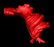
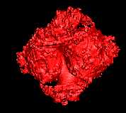
3D Mandelbrot. - Degree = 4, Iterations = 6,
Triangles = 1,502,808 |
|
 |
|
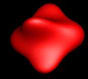
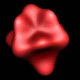
3D Mandelbrot. - Degree = 3, Iterations = 5,
Triangles = 251,000 |
|
 |
|
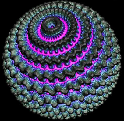
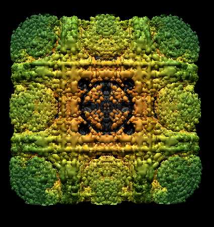
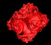
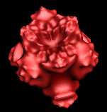
3D Mandelbrot. Degree = 32, Iterations = 2,
Triangles = 12,720,000 |
|
 |
|
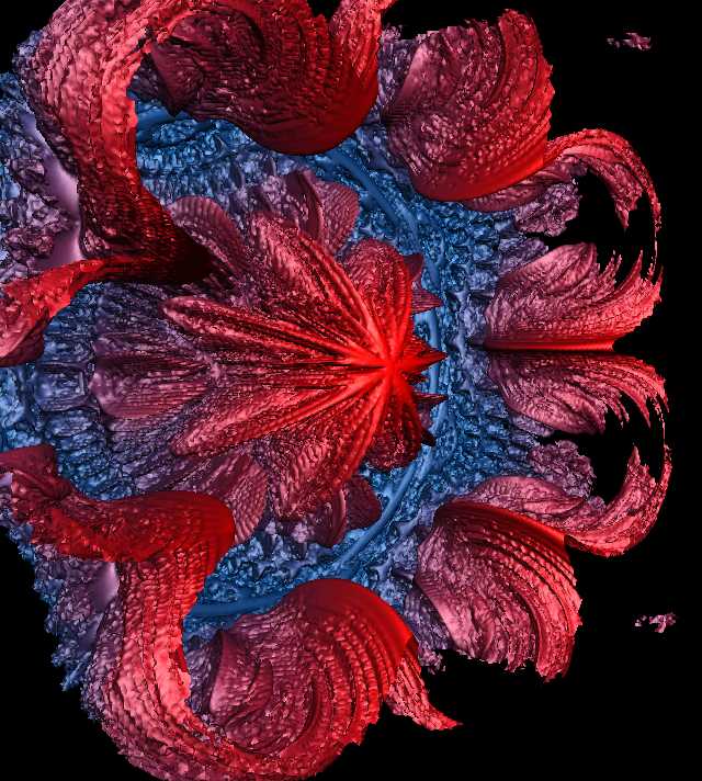
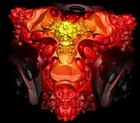
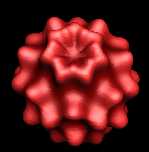
3D Mandelbrot. - Degree = 8, Iterations = 6,
Triangles = 2,038,112 |
|
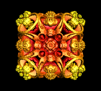
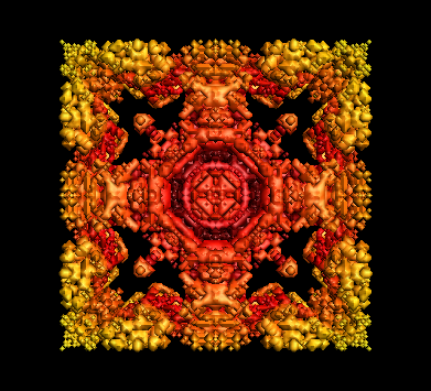
Mandel Box Images |
|
 |
|
Mandel Box - Scale -1.7 |
|
 |
|
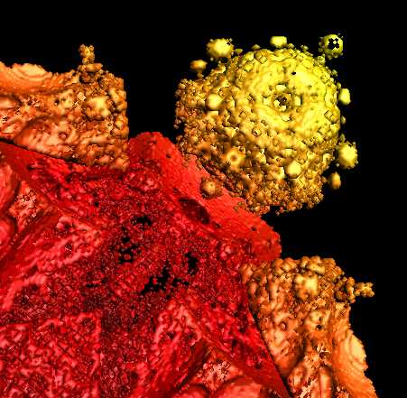
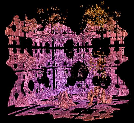
Mandel Box - Scale = 2.2 1,670,928 Triangles |
|
 |
|
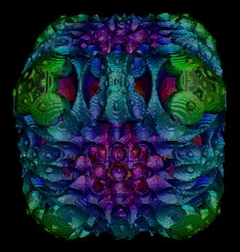
Mandel Box - Scale = -1.7 2,931,245 Triangles |
|
 |
|
Mandel Box - Scale = -2.1 Triangles = 640,735 |
|
 |
|
Mandel Box - Scale = 2.2 Triangles = 1,784,248 |
|
|
3D Mandelbrot Algorithms
and Math |
|
|
|
2D Mandelbrot. |
|
The 3D
Mandelbrot is similar to the 2D Mandelbrot, so
it is useful to review how the 2D version works.
In the 2D Mandelbrot, you are trying to find out
if an X,Y point is a part of the Mandelbrot set.
To do this, you plug the X,Y coordinates of the
point into an equation that tests if the point
is in the set. Points that are in the set are
usually colored black; points that outside the
set are colored according to how many iterations
it took to find out it was outside the set.
The equation that tests a point
looks like this: |
 |
Z' = Z^2 + C
This equation is processed
repeatedly. Every time you process the equation,
a new value of Z is calculated, which is
designated Z'. This new point will be a certain
distance from the center, or origin, of the image. If the
distance of the new Z-value goes toward
infinity, then the point we are testing is not
part of the Mandelbrot set. We know that a value
is going toward infinity if the distance exceeds
two. Once it exceeds two, the distance will
continue to get larger and larger and eventually
go to infinity, so there is no need to test the
point further.Any point
that is outside the set is colored according to how many iterations it took to
discovered it was going to infinity. On the
other hand, if the new value for Z never heads
toward infinity, the point we are testing is
part of the Mandelbrot set, and we color it
black.
Complex Numbers. The one
complication is that Z and C are
complex numbers. In other words, Z
and C have two components to each of them. For
simplicity, we'll use vector notation and label
them X and Y, so Z and C really look like this:
Z = Z.X + i*Z.Y
C = C.X + i*C.Y
This means the
math operations are more complicated than
they look:
Z.X' =
(Z.X * Z.X) + (Z.Y * Z.X) + (Z.X * Z.Y) -
(Z.Y * Z.Y) +
C.X
Z.Y' = (Z.X * Z.X - Z.Y * Z.Y) + (Z.X * Z.Y +
Z.Y * Z.X) + C.Y |
We can simplify the operation
algebraically so the expanded equations look
like this:
Z.X' = Z.X^2 -
Z.Y^2 + C.X
Z.Y' = 2 * Z.X * Z.Y + C.Y
The X and Y components of
these complex numbers are used as the
coordinates for points in the image. As a
result, you can now plug the X,Y
coordinates of the point you want to test into C.X
and C.Y
and then repeatedly process the equation to see
what happens. Here is some Pascal code that
performs the operations:
C.X:=X;  C.Y:=Y;
Z.X:=0;  Z.Y:=0;
for Count:=0 to ColorLimit-1 do
	begin
	if Sqrt(sqr(Z.X) + sqr(Z.Y)) > 2 then break;
	Z.Y:=2 * Z.Y * Z.X + C.Y;
	Z.X:=sqr(Z.X) - sqr(Z.Y) + C.X;
	end;
if Count < ColorLimit then ColorPoint(X,Y,Colors[Count]);
|
The expression
Sqrt(sqr(Z.X) + sqr(Z.Y))
calculates the distance from the origin. If it exceeds
2, we
know the point is not in the set, and we can quit
without wasting any more time. Since we only
color points that lie outside the set, the Count
value gives us a way to choose a color. However,
if the Count value reached the maximum number of
colors without exceeding 2, the point must be in
the set and we can leave the color black by not
plotting it.
There are lots of ways to
optimize the algorithm to improve its speed. For
example, it is not necessary to calculate the
actual distance. You can use the
square-of-the-distance and eliminate the square root
operation:
if (sqr(Z.X) + sqr(Z.Y))>4
then break;
|
|
3D Mandelbrot |
|
Rotations. Daniel White's discovery is based
on the fact that the 2D Mandelbrot can be
thought of as a series of rotations on a plane.
He thought that he might be able to find a
satisfying 3D Mandelbrot if he extended the
rotations to 3D. In other words, he began
experimenting with rotations in a sphere. I
won't go into the details here, but Daniel White
does an excellent job of explaining this
on his web page.
Here is the code that performs
the 3D Mandelbrot: |
C.X:=Point.X;
C.Y:=Point.Y;
C.Z:=Point.Z;
for I:=0 to Iterations-1 do
	begin
	r := sqrt(C.x*C.x + C.y*C.y + C.z*C.z );
	theta := arctan2(sqrt(C.x*C.x + C.y*C.y) , C.z);
	phi := arctan2(C.y,C.x);
	P:=IntPower(r,Degree);
	New.x := P * sin(theta*Degree) * cos(phi*Degree);
	New.y := P * sin(theta*Degree) * sin(phi*Degree);
	New.z := P * cos(theta*Degree);
	C:=VectorAdd3D(New,C);
	Result:=sqrt(sqr(C.x)+sqr(C.y)+sqr(C.z));
	if Result>1 then break;
end; |
| As
you can see, the algorithm is similar. As
before, you plug a 3D coordinate of the point
you wish to test into C and iterate through the
equation until you exit. You can exit in two
ways: 1) You may exit
because C exceeds 1 indicating that the process
is heading for infinity and there is no point in
continuing. This indicates that the point is
outside the surface of the 3D Mandelbrot.
2.) You may exit because
you've hit the Iteration Limit without exceeding
1. This indicates the point is inside the
surface of the Mandelbrot.
|
|
|
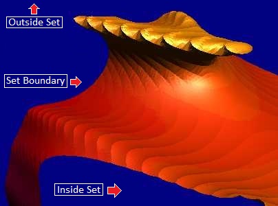
Sufaces.
The big difference between the 2D and 3D
Mandelbrots is that we are not interested in
coloring points that sit outside the set. In
this case, we are interested in displaying the
3D surface that precisely defines the boundary
between points that are inside and outside the set.
One way of doing this is with
ray tracing. If you are
ray tracing, you simply
test points along the path of the ray until the
test shows you have hit the 3D surface.
Marching Cubes. Since I
wanted to generate true 3D Surfaces, I needed to
use a different technique. Generating a 3D mesh
to model the surface is a bit complicated. |
 |
|
You can't just test every
point around the 3D Mandelbrot set. It would be
computationally intensive and waste lots of time processing points that are no where near
the set boundary.
The solution is to use the "Marching
Cubes" algorithm. The algorithm divides the
3D space up into a series of cubes. You then
test each cube to see if the surface falls
inside the cube. If it does, you interpolate the
location of the boundary and generate triangles
from the points of intersection with the cubes.
The smaller the cube, the more accurately the
mesh approximates the surface, so you can easily
adjust the resolution of the mesh by making the
cubes bigger or smaller. |
|
|
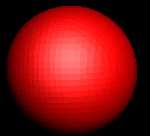
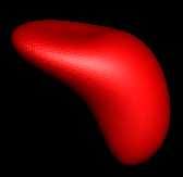
Degree and Iterations.
If you look at the sample code above, you will
see that the 3D Mandelbrot algorithm has two
parameters that control its appearance: Degree and
Iterations. The Degree
variable controls the fundamental shape of the
Mandelbrot. The Iterations
variable controls the amount of the fractal
complexity of the surface of the set.
The table and images below
show how the Degree and Iterations interact to
produce different fractals: |
| |
Interations-1 |
Iterations = 4 |
Iterations = 6 |
|
Degree = 1 |
|
|
|
|
Degree = 2 |
|
|
|
|
Degree = 3 |
|
|
|
| |
Iterations = 1 |
Iterations = 2 |
Iterations =
5 |
|
Degree = 4 |
 |
 |
 |
|
Degree = 8 |
 |
 |
 |
|
|
Mandel
Box |
|
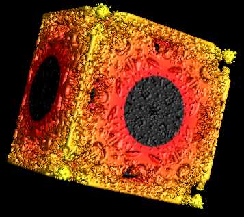
Mandel Box. The
Mandel Box is another hyper-complex, 3D-Fractal invented
by
Tom Lowe in
2010, about a year after the Mandelbulb
was discovered. It is similar to the
other fractals, but uses folding
and scaling operations to
create a whole different genre of
fractals. Here are some details:
The equation for the
Mandel Box looks like this:
Z = BallFold( BoxFold(Z) ) * S + C
C = The 2D or 3D point
that is being tested.
S = Floating point scaling value.
Z = A 2D/3D point that is initially set
to zero.
BoxFold = A square folding function.
BallFold = A spherical folding function.
As before, the formula
is iterated and tested to see if the
Z-distance
starts moving towards infinity.
|
 |
|
Folding. The
key to the Mandel Box is a series of
folding operations where the points are
folded back on themselves in various
ways.
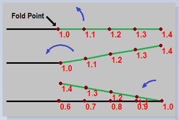
Box
Folds.
The Box Folds fold the points back on
themselves along straight lines. To
create the fold, we check to see if a
point is beyond the Fold Point and if it
is, we fold it back by subtracting. For
example, here is the code to do this for
the X-Axis:
if X
> 1 then X := 2 - X
The diagram to the
right illustrates the process. If the
X-value of a point were at 1.4, it would be folded
back until it is repositioned at 0.6. |
 |
The same process is
performed on the negative X-Axis so that
any point less than -1 is folded back
toward the origin. Likewise, the same
operation is performed on the Y- and
Z-Axes. Taken together, the operation
folds the points in a box-like pattern.
The animation to the right
shows the folding operation on a 2D
grid. You can see the grid being folded
along the 1 and -1 lines for both the X
and Y axis. (In the actual operation,
the fold is carried out all at once, so
you don't see the fold go through 180
degrees of rotation.
Here is sample
code that performs the Box Fold: |
|
|
procedure BoxFold(var Pnt: T3DVector);
begin
if Pnt.x > 1 then Pnt.x := 2 - Pnt.x
else if Pnt.x < -1 then Pnt.x := -2 - Pnt.x;

if Pnt.y > 1 then Pnt.y := 2 - Pnt.y
else if Pnt.y < -1 then Pnt.y := -2 - Pnt.y;

if Pnt.z > 1 then Pnt.z := 2 - Pnt.z
else if Pnt.z < -1 then Pnt.z := -2 - Pnt.z;
end;
|
|
Ball Fold.
The next step is a more complex fold
applied on top of the Box Fold. Instead
of folding along a line, it is folded
along the radius of two circles. The
circles are designated by their radii.
The larger circle is called the Fixed
Radius and the smaller circle is called
the Min Radius.
To accomplish the fold,
all points inside the Min Radius are
stretched so the inner radius is
expanded out to 2. This is accomplished
by multiplying each point inside the
radius by 4. To see how
the stretching is accomplished, here are
examples of different radii multiplied
by 4:
0.5 X 4 = 2.0
0.4 x 4 = 1.6
0.3 x 4 = 1.2 |
0.2 x 4 = 0.8
0.1 x 4 = 0.4
0.0 x 4 = 0.0 |
|
 |
In order to fold the points
along both radii, the points between the
Min Radius and Fixed Radius are flipped
over and stretched. The diagram below
shows the process. The blue line shows
the points inside the Min Radius. The
green line shows the points between the
Min Radius and the Fixed Radius. The red
line shows points beyond the Fixed
Radius. As you can see in the bottom
drawing, the blue line has been
stretched and the green line has been both
flipped and stretched. |
|
 |
const FixedRadius = 1.0;
const MinRadius = 0.5;
const RadiusRatio = sqr(FixedRadius) / sqr(MinRadius);


procedure BallFold(var Pnt: T3DVector);
var Radius,RF: double;
begin
Radius := sqrt(Sqr(Pnt.X) + Sqr(Pnt.Y) + Sqr(Pnt.Z));
if Radius < MinRadius then
	begin
	Pnt.X := Pnt.X * RadiusRatio;
	Pnt.Y := Pnt.Y * RadiusRatio;
	Pnt.Z := Pnt.Z * RadiusRatio;
	end
else if Radius < FixedRadius then
	begin
	RF := Sqr(FixedRadius) / Sqr(Radius);
	Pnt.X := Pnt.X * RF;
	Pnt.Y := Pnt.Y * RF;
	Pnt.Z := Pnt.Z * RF;
	end
end;
|
|
The code above shows the
Ball Fold operation. The code transforms
one point, folding it as necessary.
First, the distance from the origin is
calculated, which gives you a Radius. If
the radius is less than Minimum Radius,
the point is multiplied by a constant,
effectively stretching all points inside
the inner circle. If the point is
between Minimum Radius and Fixed Radius,
the point is multiplied by a variable
value that decreases as the radius
approaches the Fixed Radius.
This effectively folds
the points over the Fixed radius. Most
people use constant values for the Fixed
Radius and Minimum Radius of 1.0 and 0.5
respectively. Using those values, you
can simplify the code a bit. RadioRatio
becomes 4 and RF becomes 1/Radius^2. |
 |
|
The animation to the right shows the ball-fold process in two dimensions. The
colored "bulls-eye" shows the two radii,
with the blue circle showing the Minimum
Radius and the light-green circle
showing the Fixed Radius. |
Scaling. The third step in the
process is scaling. Each component of a
point is multiplied by a scale factor. If
the scale factor is greater than one, all the
points are expanded away from the
center. If the scale value is less than
one,
all the points contract toward the
center. Negative factors flips the
points from positive to negative or
negative to positive. The animation to the
right illustrates the scaling process.
The animations show the folding and
scaling in a smooth, continuous
operation to visually illustrate the
process. For example, the animations
show the software slowly bending the
points until the fold is completed. The
actual folding and scaling process
is carried out all at once. |
 |
|
Escape. The
folding and scaling operations are
repeated for an individual point until
it is clear whether the point is a part
of the set. This determined by whether
the point moves beyond a certain limit
after several iterations.
The code to the right shows the process.
After the Box Fold, Ball Fold and
Scaling are done, the result is added to
the test point C. Next, the magnitude
of the new point is calculated. This
will be the distance from the origin to
the point. If the distance exceeds the
Escape value, the point is outside the
set. If the point makes it through all
iterations without its distance
exceeding the Escape value, the point is
inside the set.
The full code for
processing one point in the Mandel Box
set is available
here. |
var Escape: integer = 4;
var Iterations: integer = 16;
Point:=MakePoint(0,0,0);
Inside:=False;
for Iter:=0 to Iterations-1 do
	begin
	BoxFold(Point);
	BallFold(Point);
	Scale(Point);
	Point:= VectorAdd(Point,C);
	Len := Magnitude(Point);
	if Len > Escape then exit;
	end;
Inside:=True; |
Scale Values.
The most important parameter in the Mandelbox Algorithm is the Scale. Small
changes in the scale, produce very
different Mandelbrot sets. Negative
values also produce interesting effects.
Experimenting with different scales can
produce surprisingly different results.
The images to the right
show Mandelbrots sets derived from
different scales. The top image shows a Mandelbox generated with a scale of 2.
The bottom image shows a scale of -3.
Another commonly used scaled is -1.7 |
 |
|
Scale = 2 |
 |
|
Scale = -3 |
|
|
|
|
|